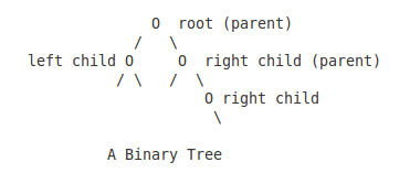
My Octopress Blog

A blogging framework for hackers.

Common Subexpression Elimination (CSE) by GCC

Test Program

    main()
        {
             int i, j, k, r;
             scanf(“%d%d”, &i, &j);

             k = i + j + 10;
             r = i + j + 30;  

             printf(“%d %d %d\n”, k, r);
        }

Assemly Code

AT&T format of assembly code is used.
  
    main:
            pushl   %ebp
            movl    %esp, %ebp
            andl    $-16, %esp
            subl    $32, %esp
            leal    24(%esp), %eax
            movl    %eax, 8(%esp)
            leal    28(%esp), %eax
            movl    %eax, 4(%esp)
            movl    $.LC0, (%esp)
            call    scanf
            movl    28(%esp), %edx
            movl    24(%esp), %eax
                leal    (%edx,%eax), %eax
                addl    $10, %eax
                movl    %eax, 20(%esp)
            movl    28(%esp), %edx
            movl    24(%esp), %eax
                leal    (%edx,%eax), %eax
                addl    $30, %eax
                movl    %eax, 16(%esp)
            movl    16(%esp), %eax
            movl    %eax, 8(%esp)
            movl    20(%esp), %eax
            movl    %eax, 4(%esp)
            movl    $.LC1, (%esp)
            call    printf
            leave
            ret

The two blocks in bold represents the evaluation of ‘k’ and ‘r’ in the test program respectively.
The ’leal    (%edx,%eax), %eax’ command adds the two values in the ‘edx’ and ‘eax’ and stores the result in ‘eax’. The ’addl’ command adds a constant to the value in the ‘eax’.
Here, both ‘leal’ and ‘addl’ are called two times, for the evaluation of ‘k’ and ‘r’ respectively.

 After optimization as:
    gcc -S -O3 -fomit-frame-pointer opt2.c
    less opt2.s

    main:
            pushl   %ebp
            movl    %esp, %ebp
            andl    $-16, %esp
            subl    $32, %esp
            leal    24(%esp), %eax
            movl    %eax, 8(%esp)
            leal    28(%esp), %eax
            movl    %eax, 4(%esp)
            movl    $.LC0, (%esp)
            call    scanf
                movl    24(%esp), %eax
                addl    28(%esp), %eax
                movl    $.LC1, (%esp)
                leal    30(%eax), %edx
                addl    $10, %eax
            movl    %edx, 8(%esp)
            movl    %eax, 4(%esp)
            call    printf
            leave
            ret

Here, what is seen to be done is:
1)
 
‘i’ in the test program stored in ‘eax’


2) ‘j’ added to ‘eax’


        Now ‘eax’ contains ‘i’ + ‘j’.


3) ‘r’ is obtained as ” 30 + the value in ‘eax’ ”


4) ‘k’ is obtained by adding 10 to the value in ‘eax’

Observation is:
        ‘i’ + ‘j’ was evaluated only once !

Common Subexpression Evaluation (CSE)

As observed, CSE is an optimization technique employed by the compiler, when the same subexpression is present in more than one expressions.

It is as if the subexpression is evaluated first, and the result is stored in a temporary variable. For all further calculations where this subexpression was a part originally, the value of this newly created temporary variable will be used.
In the test program used above, the so evaluated subexpression is ’ i + j ’.

Also, CSE is performed only when, in that environment, the cost to use such a temporary variable is lesser than the cost to perform the operations in the subexpression itself. Here, the operation is ‘+’. 

Depicting Function Inlining by GCC

Inline Function

In C, if a particular function used has only a few lines in its body, and if the optimization level is set to 03 (preferably), some unexpected changes can be observed about how gcc handles this function.

What the compiler will do is that it replaces the call for this function, with the actual code of the function, called inlining.

The limit on the number of lines below which inlining is performed, strictly depends upon the gcc heuristics.

This is not all. In  the extreme case, if the small function mentioned above only does something like calculating a value after taking an input, then gcc will evaluate the function call, calculate the value, and directly paste it in the program instead of the function call itself.

Sweet, isn’t it?  

Test Program


    int sqr(int x)
        {
            int a;
            return x*x;
        }

    main()
        {
            printf(“%d\n”, sqr(10));
        }

Assembly Code

To view the assembly code.
    gcc -S -fomit-frame-pointer opt1.c

    less opt1.s


The assembly code is:
    sqr:
            subl    $16, %esp
            movl    20(%esp), %eax
            imull   20(%esp), %eax
            addl    $16, %esp
            ret
          
    main:
            pushl   %ebp
            movl    %esp, %ebp
            andl    $-16, %esp
            subl    $16, %esp
            movl    $10, (%esp)
            call    sqr
            movl    %eax, 4(%esp)
            movl    $.LC0, (%esp)
            call    printf
            leave
            ret
          
On optimization,

    gcc -S -O3 -fomit-frame-pointer opt1.c

        less opt1.s

The new code is:

    sqr:
            movl    4(%esp), %eax
            imull   %eax, %eax
            ret
    main:
            pushl   %ebp
            movl    %esp, %ebp
            andl    $-16, %esp
            subl    $16, %esp
            movl    $100, 4(%esp)
            movl    $.LC0, (%esp)
            call    printf
            leave
            ret

Here, the function sqr( ) does something very simple, and the input to the function is statically assigned. It means that the value of the input (10) will never change during runtime. Hence, the compiler will optimize the program even further, to the extreme that the square of 10 will be evaluated and the result pasted in the program instead of the original call to the function sqr( ).  

User Mode Linux Built From Scratch !!!

Linux From Scratch
“Linux From Scratch (LFS) is a project that provides you with step-by-step instructions for building your own custom Linux system, entirely from source code.”
Homepage is : http://www.linuxfromscratch.org/ .

Use Mode Linux
“User-Mode Linux is a safe, secure way of running Linux versions and Linux processes. Run buggy software, experiment with new Linux kernels or distributions, and poke around in the internals of Linux, all without risking your main Linux setup.
User-Mode Linux gives you a virtual machine that may have more hardware and software virtual resources than your actual, physical computer. Disk storage for the virtual machine is entirely contained inside a single file on your physical machine. You can assign your virtual machine only the hardware access you want it to have. With properly limited access, nothing you do on the virtual machine can change or damage your real computer, or its software.”

UML - The kernel on top of a kernel 

To get the complete idea, it is true that the UML kernel can be booted and shutdown from your Linux system, just like another application. It will not cause your Linux system to halt in any way.

How is the required privilege levels setup for the UML kernel?
The privilege levels in a Linux system ranges from 0 (ring 0) to 3 (ring 3). Ring 0 gives you complete power. You can change the contents of any register, do anything. Ring 3 is the user mode. It also has the lowest privilege.

This is the same in the UML kernel too.

Can a C code get privilege level 0?
Yes it can. Through system calls. But it cannot be allowed just like that. Allowing a C code full control will be like allowing viruses to grow in Linux! The C code must be able to make system calls, and simultaneously not be the one who is in possession of the control flow.

This is the specific design technique employed in Linux. When a system call occurs in a C code, there will be a switching from ring 0 to ring 3. It will be simultaneously accompanied with transfer of control from the C program to the Linux kernel. No hassle there.

Thus, total safety is ensured.

How is the UML kernel designed then?
A Linux kernel comprises of two parts:
1) the hardware dependent part - specifically, everything inside the ’arch
                                                    folder in the kernel source code.
2) others

What is done in the UML kernel is that:
1) take away all the hardware dependent part of the kernel.
2) simply replace it with the system calls of the kernel layer below
    it (pure C code).
    (the UML kernel will behave just as an application)

Consider a sample executable binary ‘a.out’ compiled inside the UML kernel, from a sample file ‘a.c’.

Fig 1. The kernel layers

a.out makes a system call
e.g. read( )


replace a.out’s call with the address of
its own read( )


The mechanism:
The UML kernel uses ptrace( ) to freeze ‘a.out’, the moment it invokes a system call. Then, the address of this function call is replaced with a corresponding system call address that is part of the UML kernel itself.

Everything works fine, in a cute way.

Compiling and Booting the UML kernel

While compiling the kernel, just add an extra parameter ’ARCH=um’ to all the steps outlined in the Linux kernel README.
After compilation, an executable binary called ’linux’ will be created.

Assuming ‘linux’ is present in your current directory, to boot into the UML kernel give the command as:
    ./linux ubda=< path of the filesystem >

where filesystem can be a physical partition, or one created with the dd and mkfs/mke2fs commands.

Some Snapshots

‘Make’ing Glibc 
Fig 2. Running ‘make’ for glibc
 ‘Configure’ing Bash
Fig 3. ‘Config’uring Bash
Linguistic Perl 
    The configuration settings for Perl, created by Larry Wall, was the most “linguistic” out of these!  Some excerpts are:


Fig 4. Excerpts from the ‘configure’ settings for Perl5

Man pages


    These had a make install’ with one of the shortest SBU, and looked a bit of a variety too!

Fig 5. ‘make install’ of man pages
Bash without name !
    During the process, there is a time when ‘chroot’ is used to completely move into the LFS installation and start using the programs already setup inside it.  At this point, the Bash will be setup without creating the /etc/passwd file. Now the Bash will say that it has no name !
Fig 6. Bash without /etc/passwd
After the Bash has been recompiled and installed properly with respect to the LFS system, and the /etc/passwd file created, the Bash prompt reverts back to normal.
Fig 7. Bash after recompiling and creating /etc/passwd
Booting in …
Fig 8. Booting into the UML kernel
Powering off …
Fig 9. Powering off the UML kernel

The AVL Tree

BINARY TREE

A binary tree is a tree data structure in which each node has atmost two child nodes. The child nodes may contain references to their parent nodes. There is a root node, which has atmost two children but no parent.

According to Graph Theory, a binary tree can be also said to be a connected, acyclic graph data structure, with a maximum degree of three for each vertex.

TERMS ASSOCIATED WITH A BINARY TREE
  • The root node of a tree is the node with no parents. There is at most one root node in a rooted tree.
  • A node with no children is called leaf node.
  • The depth of a node is the length of the path from the node to the root. All nodes at the same depth are said to be in the same level. The root node is at level 0.
  • The height of a tree is the length of the path from the node which has the highest depth, to the root node.
  • The children of the same parent are called siblings.
  • A node is an ancestor of another node, if it comes in the path traced from the other node to the root.
  • A node is the descendant of another node, if it is the child of the other node, at some level from it.
  • The size of a node is the number of descendants it has including itself.
  1. A perfect binary tree is a full binary tree in which all leaves are at the same depth or same level. (This is ambiguously also called a complete binary tree.)
  2. A complete binary tree is a binary tree in which every level, except possibly the last, is completely filled, and all nodes are as far left as possible.
  3. A balanced binary tree is where the depth of all the leaves differs by at most 1. This depth is equal to the integer part of log2(n) where n is the number of nodes on the balanced tree.
BINARY SEARCH TREE

A binary search tree is a binary tree in which the numerical value of the data field of the left child is lesser than that of the parent, which is in turn lesser than that of the right child. In short,
(data of left child) < (data of parent) < (data of right child) [numerical value of data is taken]
For example,

Here, in both the trees, data is input in the same order, i.e, 34, 43, 56, 21. Searching in the binary tree is evidently very easier in the BST, hence the name binary search tree.

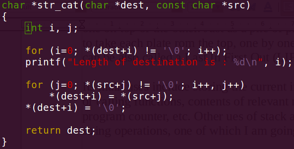
Each node in a binary search tree can be represented by a structure in C, created with the ‘struct’ keyword, typically named ‘node’. In the most simple case, the data field is taken as an integer. There are three pointers associated with each node, whose typical names can be parent, lchild and rchild, of type ‘struct node’ itself. These three pointers also make the structure ‘node’ a self-referential data structure. Obviously, the parent pointer in the structure representing the root node, will be NULL.

The definition for each node will be:
struct node {
int data;
struct node *parent;
struct node *lchild;
struct node *rchild;
};

The names for the fields are self explanatory, and arbitrarily taken.
(The ‘parent’ pointer points to the parent of a node. It is necessary in an AVL tree only.)

BASIC FUNCTIONS FOR THE BST

Since the binary search tree is a dynamic data structure, the malloc() and free() C standard library functions are used to allocate memory for new nodes while insertion, and to deallocate memory while deleting nodes, respectively. Only the following basic functions are needed to implement the full functionalities associated with a BST.

Constructor -> For creating a new node in the BST
Insert -> For inserting the new node into the BST and
                                           setting up the links
Traverse Inorder -> For inorder traversal through the BST
                                           (for each node, print LnR)
Traverse Preorder -> For preorder traversal through the BST
                                           (for each node, print nLR)
Traverse Postorder -> For postorder traversal through the BST
                                           (for each node, print LRn)
Find                        -> For returning the node whose data field is the
                                            given numerical value
Delete -> For deleting a node from the BST.

where ’n’ denotes the current node, ’L’ the left child, and ’R’ the right child. (thanks to Shijith for this one …)

N.B. For deletion, if the node is a leaf, just delete it. Otherwise, if the node
         has a right child, replace the node with its successor node in the
         inorder representation of the BST. Else, replace the node with its
         predecessor in the same inorder representation.

BALANCING A BST

The BST seems efficient in searching for a particular data. But it is not so always. When there are large number of nodes, there is the possibility that a devastating situation, as shown below, may occur.

In the second BST, data was input in the order 21, 20, 34, 37, 43, 56. Hence, the structure. According to the BST terminology, a structure like this is said to be unbalanced.

N.B. A BST is said to be balanced, when the depth of any two leaves in
         the BST differs atmost by 1. Also, a balanced tree will be
         theoretically more efficient in all situations, while an unbalanced tree
         will be not.

Why is an unbalanced BST inefficient? For mainly two reasons.
1) The time complexity for searching some data values becomes much
    greater than expected. For example, in the first BST, 43 can be found in
    two steps of traversal. In the second one, it takes an unexpected 4 steps.
    For very large BSTs, the time complexity increases drastically.
2) The lesser the number of levels in the tree, the more efficient the storage.
    When operations like deletion are performed on large BSTs, there is
    a high possibility that the actual addresses of the nodes are spread out
    over a large area of the storage memory (secondary memory).

How to balance a BST?
There are many techniques available, but in all of them, the simple rule is to keep the difference between the depth of any two leaves atmost 1. The BST can be balanced at a particular point in time as desired, or it can be done while insertion into and deletion from the BST. Such BSTs that do “balanced” insertion and “balanced” deletion are called self-balancing binary search trees.

THE AVL TREE

The AVL tree is one of the many kinds of a self-balancing binary search tree. It was invented by G. M. Adelson-Velskii amd E. M. Landis.

Short Bio of the Inventors
G. M. Adelson-Velskii
Georgy Maximovich Adelson-Velskii, was born on 8 January, 1922 in Samara, Russia. He is a Soviet mathematician and computer scientist. Along with E.M. Landis, he invented the AVL tree (“AV” in “AVL” tree stands for Adelson-Velskii) in 1962.
In 1965, he headed the development of a computer chess program, which evolved into Kaissa, the first world computer chess champion.
He currently resides in Ashdod, Israel.

E. M. Landis
Evgenii Mikhailovich Landis, was born on October 6, 1921, in Kharkiv, Ukrainian SSR, Soviet Union. He was a Soviet mathematician who worked mainly on partial differential equations.  He studied and worked at the Moscow State University.
With Georgy Adelson-Velsky, he invented the AVL tree datastructure (“L” in “AVL” stands for Landis).
He died in Moscow on December 12, 1997.

The Technique

The BST can be easily remodelled into an AVL tree by adding some extra functions that perform balanced insertion and balanced deletion. Some other helper functions that perform some trivial tasks are also needed. The balancing is done by a technique called “rotation”.

What is rotation?
It can be best illustrated only pictorially. There are two ways to rotate.

i. 
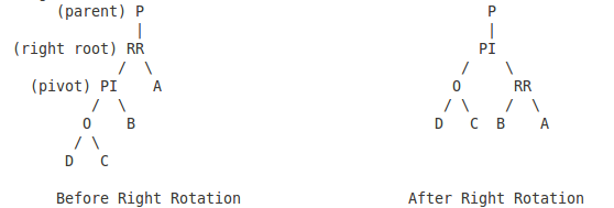
Right Rotation                    

What happened simply looks as if:
1) node 34 was kept fixed as a “pivot”.
2) 34’s right child was rotated clockwise about the pivot (node 34 here).
3) there is a change in some links of 34 and 43.

On generalising,

ii.
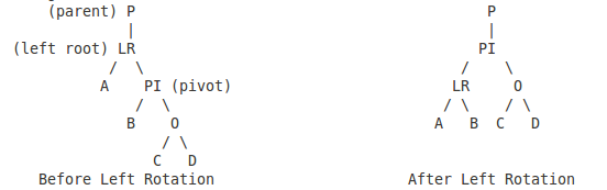
Left Rotation                    

What happened simply looks as if:
1) node 37 was kept fixed as a “pivot”.
2) 37’s left child was rotated anti-clockwise about the pivot (node 37 here).
3) there is a change in some links of 21 and 37.

On generalising,

N.B. In both cases, the structure of the original BST will be changed to
         that after the rotation. The rule for a balanced tree will be obeyed
         in both the new structures.

Above mentioned are the two ways to perform rotation. When and how many times to perform them depend on the actual arrangement of the nodes in the BST. There are four distinguishable imbalance patterns which occur repeatedly in a BST strucuture. These four patterns are recognized by finding out the “balancing factor” for each node. According to the balancing factor thus obtained, the proper sequence of rotations can be initiated.

What is the balancing factor?
For any node in the BST, its balancing factor is given as:
BF (node) = (height of its left subtree) - (height of its right subtree)

(It can be taken the other way round too, but appropriate sign changes have to be made in the balancing factor of nodes.)  
BF (node 43) = +2
BF (node 34) = +1
BF (node 21) = +1
BF (node 20) = 0 (leaf)

The balancing factor of any node in a balnced BST will be an integer, in the range -1 to +1, including them. If the balancing factor of a node is found to be -2 or +2, it indicates that the BST is unbalanced at that node.
Next, the proper imbalance pattern is identified. Once it is done, the appropriate sequence of rotations are performed.  

THE FOUR CASES OF IMBALANCE

For any number of nodes in a BST, only 4 patterns occur repeatedly. They are classified as the four cases according to which different sequences of left or right rotation or both must be performed. The four cases are:

    LEGEND:
1 - node with BF +2 or -2, indicating need for rotation
parent              - the parent link of node 1
lroot and rroot - the nodes which get “rotated” during each of the left
                             or right rotations respectively
pivot                 - the pivot node in a rotation

From the above figure,
LEFT - LEFT CASE : BF of a node is +2, BF of its left child is +1 or 0
LEFT - RIGHT CASE : BF of a node is +2, BF of its left child is -1
RIGHT - RIGHT CASE : BF of a node is -2, BF of its right child is 0 or -1
RIGHT - LEFT CASE : BF of a node is -2, BF of its right child is +1

Also,
LEFT - LEFT CASE : 1 right rotation
LEFT - RIGHT CASE : 1 left rotation, then 1 right rotation
RIGHT - RIGHT CASE : 1 left rotation
RIGHT - LEFT CASE : 1 right rotation, then 1 left rotation

AVL-SPECIFIC FUNCTIONS

Balancing Factor -> Finds the balancing factor for the given node.
Left Rotation -> Perform left rotation, given a “pivot” and “lroot”.
Right Rotation -> Perform right rotation, given a “pivot” and “rroot”.
Balance -> Check balancing factor of given node. If the tree is
                                       unbalanced at this node, identify the imbalance
                                       pattern and perform rotation.
Balanced Insert -> Insert a new node, then travel from its parent to the
                                       root, calling Balance() for each node in the path.
Balanced Delete -> Delete the node, then travel from its parent to the
                                       root, calling Balance() for each node in the path.
                                       If the deleted node was not a leaf, the path starts
                                       from the replaced node itself.
                                    
Special Conditions to be Checked while Retracing in Balanced Deletion

If at some node, its BF is:
+1 or -1 : it indicates that the height of the subtree has remained unchanged,
                and retracing can stop.
0            : height of the subtree has decreased by 1, and retracing needs to
                continue.
+2 or -2 : needs rotation.
                If BF of the node after rotation is 0, continue retracing since
                height of this subtree has again decreased by 1.

N.B. In insertion, if the BF of a node after rotation is 0, it indicates that the
         height of that subtree has remained unchanged, contrary to the similar
         situation while deletion.

CONCLUSION
Once the above extra functions are defined, the BST will be remodelled into an AVL tree.

HOWTO Smash Your C Stack and Learn More !!!

Stack is an abstract data type (ADT) in C. It is a memory visualization, where the memory contents are put inside one on top of the other. Just as a pile of plates. We have to take each plate rom the top, one by one. Hence, a stack can be also called a Last In First Out (LIFO) structure.

Its main uses include storing the current instruction address of a program when it calls another function, contents of relevant registers like the program counter, etc. Other uses of stack are seen while performing string operations, one of which I am going to use now.


A simple implementation of builtin strcat()
———————————————————
The program can be as follows:
Fig 1. The pseudo code for strcat()


Its time to play with the test data. Initially,
Fig 2. Initial test data


The output will be printed graciously as,
Fig 3. Initial output


My name is ‘hari john kuriakose’
———————————————
It is only natural that I try to concatenate the two ‘halves’
of my name. So my new test data is,
Fig 4. Test data 2


Surprisingly, we get a peculiar output. What we see is,
Fig 5. Output for test data 2 - part I


Fig 6. Output for test data 2 - part II


Note that the length of destination (here its a) is 7. The stack will be smashed for the lengths 8 and 9 too, but not for other arbitrary lengths. Also, this behaviour is true only when length of the source (here its b) in all these cases is >1.
Fig 7. Test data 3

Fig 8. Test data 4


If the length of the source is 0 or 1, no smashing occurs.

Similarly, when concatenation is in the reverse order, the stack smashing willl occur only when the length of destination (here its  b) is 7 and length of source (here its a) is >1.
Fig 9. Test data 5


Here too, no smashing is observed when length of source is 0 or 1.


Analyzing with gdb
—————————
On analysis, the program works fine. There will be no problem till the very last line. Consider the test data is one among the problematic cases mentioned above. On exiting from main() after seeing the closing curly bracket, this odd behaviour suddenly springs up. But now, gdb informs that two more things have happened.
1. Program received signal SIGABRT, Aborted
2. 0x0012d422 in __kernel_vsyscall ()
Fig 10. gdb output - part I

Fig 11. gdb output - part II


This, is interesting. What are these things?


SIGABRT
————–
It is a signal. It is defined in signal.h . It is used to tell a program to abort. Its signal number is 6.

On some platforms, SIGIOT (signal for I/O transfer) is taken as a synoym for SIGABRT. It is also the signal a process sends itself when it calls the abort libc function, defined in stdlib.h . The SA_SIGINFO macro would be interesting too.

SIGABRT can be caught, but it cannot be trapped. When the signal handler returns, all streams must be flushed out and the program terminated. Hence, an abort function will not return. This signal is used to indicate fatal conditions in the supporting libraries, when the program cannot continue, but the main() can cleanup while it exits. Typical example is, on the failure of an assertion.

If a SIGINFO is called after the occurrence of a SIGABRT, a pointer to a structure of type ABRT_t will be returned. This strcuture contains a printable form of the ABEND code. Since SIGABRT cannot return to the point of interrupt, an attempt to do so will reissue a ABEND.


__kernel_vsyscall()
————————-
This is the method used by linuxgate.so (a part of the kernel) to make fast system calls, usually using sysenter.

The linuxgate.so is a Virtual Dynamically-linked Shared Object (VDSO), a kernel-provided shared library that helps userspace perform a few kernel actions without the overhead of a system call, as well as automatically choosing the most efficient syscall mechanism. Also called the “vsyscall page”.
This is as per the KernelGlossary.

Or, the linux gate is the actual interface between the kernel and the user space. Originally it was named linux-vsyscall.so.1, but to make it more meaningful, it was changed.

To view the linuxgate.so, print the shared library dependencies for the shell.
    ldd /bin/sh
Fig 12. The Linux gate


But the address you see there, does not actually exist. It is just a shared object used by kernel to facilitate a VDSO. To know whether your kernel is VDSO enabled, you can see the contents of a file in /proc, which contains the currently mapped memory regions and their access permissions.
    cat /proc/self/maps

Fig 13. cat /proc/self/maps - part I

Fig 14. cat /proc/self/maps - part II


In the kernel, all processes will therefore share this same object, which enables us to do a simple trick with the convert and copy ability in linux, the dd tool. On successive objdump, the ‘__kernel_vsyscall’ can be spotted. On further objdumping, the underlying ‘sysenter’ can be seen too.

What are ’system calls’?
They are the means by which a user can access the services offered by a kernel. Those services include storage, process management, etc. In C, the stubs are the interface to invoke system calls.

Is that all?
No. In a system call, the actual code running is a part of the kernel itself. It runs with a privilege level 0 (CPL 0), which is the highest level in x86 architecture. It is termed ’ring 0’. All user processes run in ring 3. Thus, to sucessfully make a system call, we have to call a ring 0 code from a ring 3 code.

What are these ’faster system calls’ ?
Originally, in the x86 architecture, all system calls were implemented as interrupts. Linux and Unix-like kernels used 0x80. For the newer members in the x86 family, it was observed that interrupting via 0x80 was getting much slower! A Pentium IV was more slower than a Pentium III in this particular respect. Intel recognized this problem early, and introduced two instructions, ‘sysenter’ and ‘sysexit’. But the hardware bugs were so plenty, they could not boast about it.

That was until Linus Torvalds came along. He was very skillful in manipulating the fact that the return point of ‘sysenter’ instruction is totally arbitrary, and he wrote some highly tricky code that ultimately came out as the solution!!! Anyways, he himself says his final solution is disgusting!

For the techier techies, 


N. B. 
———
The pseudo code can be tweaked slightly and made theoretically correct.

Elementary Analysis of TinyPython Virtual Machine v1.1

OVERVIEW
TinyPython is a minimalist implementation of Python in 64K
code, originally created by Phil Hassey. He blogs at:

It is a parser and byte-code compiler written in
TinyPython itself. It is also fully bootstrapped in the sense that
initially, TinyPy converts a Python script (.py) into a special
TinyPy byte-code format (.tpc), and this generated code is then
passed into a subset of the TinyPython source code called the
Virtual Machine, where the actual execution takes place.

One can even extend the idea that if the VM is compiled into a
low-level format adaptable to a particular microcontroller,
then the VM will reside inside that chip, and any .tpc file can
be downloaded into the chip as its input.

A basic analysis of source code for TinyPy v1.1, excluding the
byte-code compilation phase, was performed. The focus was
on the working of the TinyPy Virtual Machine, which actually
executes the byte-code.

The TinyPython source code used was downloaded from:

BUILDING TINYPY
Initially, the file listing will look like the following figure:
Fig 1. TinyPy source file contents

   Initially, the ‘build’ folder will be empty. The ‘doc’,
‘examples’ and ‘modules’ folder may or may not contain
any documents, Python scripts and batteries (or modules)
respectively, depending on the downloaded package.
The LICENSE.txt, README.txt, CHANGES.txt and
ROADMAP.txt describe the essential details of TinyPy.
The ‘setup.py’ contain the initial code to build the TinyPy
from scratch. At the terminal, type as follows:
    python setup.py linux

It is implied that you need a Python interpreter available in 
your system. The ‘linux’ option is to specify that the code will
be compiled so as to make it work in a Linux environment. 

Now, a new executable ‘tinypy’ will appear in the ‘build’ folder.
To fully bootstrap and test TinyPy, give the command as:
    python setup.py linux boot

Now, in the ‘tinypy’ folder shown above, two new 
executables, ‘tinypy’ and ‘vm’ will appear, which are the 
TinyPy parser, and Virtual Machine respectively. It can be 
noticed that new .pyc files for the corresponding .py 
files have also been generated by the Python interpreter.

The general usage and some options available are listed below:
    python setup.py command [option] [module]

64 k - build a a 64k version of TinyPy source code
blob - build a single ‘tinypy.c’ and ‘tinypy.h’


The ’py2bc.py’ script is used to convert a user-generated 
Python script into its corresponding .tpc file.
    python py2bc.py sample.py sample.tpc


Here, tinypy_path is the path (relative to current position) 
of either the tinypy executable in the ‘build’ folder, or the one
in the ‘tinypy’ folder. ‘sample.py’ is the name of the user-script.
‘sample.tpc’ is the name given for the byte-code converted file.


Finally, the generated byte-code (.tpc) is to be passed into the
VM for compilation and execution. Assuming the current 
directory as ‘tinypy’ folder, it is done as:
    vm sample.tpc

Or logically,

    gcc vmmain.c -lm ./a.out sample.tpc

The ‘vmmain.c’, present in the ‘tinypy’ folder, is the main 

function of the VM which runs and automatically links all the
other files necessary for the VM. And now the output is
obtained and displayed. For a better picture, the files actually
needed for VM are:
Fig 2. The files needed for the VM

For debugging and understanding the flow of control within
the source code, the ‘gdb’ and ‘ctags’ tools were used.
ANALYZING THE VM
A sample program ‘sample.py’:
    def add(a, b):
        c = a + b
        return(c)
    print(add(1, 9))
gives you the output:
      10

Each time the VM is invoked, a new instance of the VM is
created .
    tp_vm *tp = tp_init(argc, argv);

“Each object in tinypy is stored as a union in the C API.”
tp_obj is tinypy’s object representation.
typedef union tp_obj
{
    int type;
    tp_number_ number;
    struct{int type;int *data;}gci;
    tp_string_ string;
    tp_dict_ dict;
    tp_list_ list;
    tp_fnc_ fnc;
    tp_data_ data;
}tp_obj;

The field ‘type’ of the union indicates the type, of the object.
A type value of 1 indicates that a number is being used,
type = 2 indicates object is a string and type = 4 indicates a list.

In the sample program, a function in the VM ‘tp_add’ does the
job of adding two arguments (numbers, strings, lists) that are
passed to the function as input.
     tp_obj tp_add(TP, tp_obj a, tp_obj b)

The function definition of ‘tp_add’ contains three arguments:
   • TP -> the VM instance
   • tp_obj a -> the union variable representing the object ‘a’ in
                        the sample program
   • tp_obj b -> the union variable representing the object ‘b’ in
                        the sample program

‘a’ and ‘b’ are stored as unions and contains fields for types
such as number, strings, lists, etc.

Consider two simple lists in Python:
    a = [1,2,3]
    b = [4,5,6]

The VM uses a function ’tp_extend’ which returns a union that
contains the new (extended) list. Its ‘type’ would be 4 indicating
a list. The ‘list’ structure variable includes a pointer *val that
points to another structure ’_tp_list’.
    typedef struct _tp_list
    {
        int gci;
        tp_obj *items;
        int len;
        int alloc;
    }_tp_list;

The pointer *items as you could see is of type tp_obj and
de-referencing it would give you the union tp_obj. This
union contains a single element of the final list.

To obtain the next element of the final list:
    r.list.val -> items

would give you the address of the union.
Union containing the next element of the list = Address of 
the current union + size of each union.
   Here:
    r.list.val -> items = 0x96ca048 + 10

would give you the union that stores the next element of the
list . The size of the union is 10, in hexadecimal = 16 bytes.
Fig 3. The representation of a list

THE PATH OF ‘tp_add’
Fig 4. The backtraced path of ‘tp_add’

   While debugging, our sample program and one of the 
input data too, can be spotted as:
Fig 5. Spotting the sample program
Fig 6. Spotting one of the inputs

   The switch() inside ’vm.c’ is invoked nine times, one of
which will be the selection of case: ’TP_IADD’ and 
subsequent execution of ’tp_add’.
Fig 7. The case: ‘TP_IADD’

Another trial debugging was done with input file ‘testing.tpc’, 
whose source script was ‘testing.py’ which just added two 
numbers. Only the filename ‘testing.tpc’ was given to the 
debugger.

The VM snapshot taken while debugging, showing the 
name of the source script ‘testing.py’ and the function used
‘print(a + b)’ stored in the fields of the VM data structures,
and the conclusion to this analysis, and more details can be
found in:

Memoization

Computers are very fast machines. But the computation time
also depend on the algorithm we choose. It can happen that
if a proper algorithm is not chosen, it may take a very long
time for execution.

On writing a simple recursive fibonacci generator function for
the nth element, fib(n), we will get fine results, but only for low
values of n. This is because fib(n) has exponential complexity.
Such functions grow very fast, so fast that even for small
values of `n’ (where `n’ is the size of the input), our program
will take a long time to finish.

Memoization is the process by which we speed up the situation.
The underlying principle is to create an associative array, say  
dict, which contain keys = n, and values = fib(n). Each time a
fib(n) is called, the associative array will be checked whether it
contain the key ‘n’. If yes, just return dict[n]. Otherwise, create
a new key: value pair for dict. Thus, the number of recursion will
be drastically reduced, with this look-in-the-lookup-table policy.

Ofcourse, memoization is an upgrade to time compplexity, but
will consume space.
The implementation in Python looked like:

def memoized_fib(x):
if dict.has_key(x):
return dict[x]
else:
dict[x] = fib(x)
return dict[x]

def fib(n):
if n == 0: return 0
elif n == 1: return 1
else: return memoized_fib(n-2) + memoized_fib(n-1)

 dict = {0: 0, 1: 1}


In Python, the recursion limit is fixed by the interpreter itself. It can
be found in:
sys.setrecursionlimit(<limit>)

Now, set a very high limit, and run the code. If its high enough, u will
deplete the stack memory size (8 MB) of the C backend of your Python
virtual machine, leading to a segmentation fault there, which is
propagated back to your Python interpreter, crashing Python itself!

To Fly With the Phoenix …

Well, I must say, simplicity and brilliance is what a FOSS meet will be
all about, if you watch the proper people. For the National Conference
on Free Software And Education, September 10-12, 2010, me and
my four friends Prasanth, Remya, Sumith and Sunil geared up with a handy electronic instrument called the Phoenix(aptly named), and barged in
through the front gates. We came to know about the Phoenix from our
teacher, Mr. Pramode C. E., and beacme interested. This interest made
us to take it to the FOSS meet and do a few tricks with it, with guidance
from Pramode Sir. Some mistakes and pitfalls happened too.

First of all, whats ’Phoenix’? Its an electronic gadget with an Atmel
ATmega16 mcu inside it, with hardware peripherals including a DAC, ADC,
digital I/O pins, comparator, waveform generator, amplifier, etc,
necessray to build a simple circuit. The point? The whole Phoenix board
is set up such that a large variety of experiments from Physics can be
conducted with ease. Highly accurate measurements are thus possible.
Experiments include a simple charging-discharging cycle of a capacitor,
to alpha particle radiation measurement from a radiative source. Plus,
the board runs in C, with the computer front-end being Python. Hows
that? An ‘open hardware’, it may be called, maybe the first of its kind.

Coming back, the first day was at Tagore Centinery Hall, Calicut Town.
A banner highlighted by the face of Richard Mathew Stallman a.k.a
R. M. S. greeted us. Volunteeers and coordinators from NIT Calicut, gave
a brief picture of the schedule. Understood that, only the inaugral
ceremony with a keynote address from R. M. S. will be arranged that day.
At the far end, some tables were set up, and many free software users
were vigorously working with their laptops.

We were to see Mr. Sasikumar, the ‘R. M. S.’ of Kerala. Till then, we
were just standing their groping with our belongings, not knowing what
to do. Once we met him, the situation changed abruptly. We were greeted
with a warm, enthusiastic, polite smile, and ushered to the expo area.
The volunteers were asked to allot a table for us. Then, we became a
part of the event.

Till the original R. M. S. arrived on the scene, the expo continued. A
few people came to visit the ‘stalls’. There were students, enthusiasts,
Physics teachers, and others who came to see what Phoenix was. There
were Phoenix users among them too, who wanted to see if any newer
features have been developed for the Phoenix.

Finally, I learned that R. M. S. had arrived, and has gone inside the
Hall, while my back was turned. Soon, everyone got inside, and I saw
the guy for the first time. I was seeing a cute-in-an-odd-kind-of-way,
big, living genius. I stared at him for long, with only one thought in
mind. I had to hear his voice too. Meanwhile the guest were asked to
get on stage. R. M. S. chose a side chair, but was ushered to the
center of the dias. Later, I saw him, kneeled down on his left leg,
drinking water from a bottle, kept on a table infrot of him. Well,
everything he did seemed cute and nice. A few moments later, he simply
yawned, and I couldnt help but smile.

There were to be about 8 more felicitations before the keynote address
from R. M. S. We couldnt wait that long, we had to get to our staying
places. We reached NIT Calicut, next day by noon. We arrived before for
the lunch session and quickly set up the table. Many people came to us
during the break, to know about Phoenix. There was a Physics teacher,
who believed Physics has to be ‘touched and learned’. But i had a
counter-point that Phoenix could do things otherwise impossible in a
lab. One particular student was so excited to hear about Phoenix,
because he had been looking around for such a low cost instrument for
obvious purposes. There was a table for IIT Bombay, who had come with
their project to create spoken-tutorials for all the major free
software applications available now. Shortly after the lunch session
was over, we packed our things and got out, because we had to reach
our shelters in the same day itself.

Mistakes:
1. I didnt take photographs all through the event.
2. Didnt bring a banner or charts (showing the details of Phoenix) for
    display purposes.
3. Didnt bring a better experiment apparatus, perhaps it could have
    gained more attention.

Pitfalls:
1. We totally lost control of time. We were running for shelter to
    sleep, running to be present at the meet.
    In a nutshell, we couldnt sit for a single talk.

What we learned:
1. What to expect and what not to in a FOSS meet.
2. The feeling when someone like Dr. Prabhu Ramachandran whizzes past
    you, and you continue to stare blankly, unable to utter a single word.
3. How it is to bring ‘something’ to the meet and to bring ‘some real
    thing’ to the meet, from the fact that, we had also brought along an
    elementary study report on the TinyPy Virtual Machine v1.1.

Classes in Python

In Python, ”classes are objects too”. Let me clarify.

Let me define a sample class.
>>> class abc: pass
>>> abc
<class__main__.abc at 0xb76e341c>
It indicates that in Python, classes are not abstract!
They too take memory space.


Lets explore further.
>>> m = abc
>>> m
<class__main__.abc at 0xb76e341c>
>>> m = abc( )
>>> m
<__main__.abc instance at 0xb76e298c>
i.e, in Python, both classes and their objects are concrete.

Now,
>>> abc.p = 10
>>> abc.p
10
Classes can act as objects, as already told above!


Still further,
>>> m = abc()
>>> m.p
10
>>> m.q = 20
>>> abc.q
20
What exactly happened here?


Things to understand:
1. Here, “.” works as a search operator 
2. On querying m.p, first checks if there’s a p attribute in m
3. If not, automatically finds out type of m, then searches for p there.
4. The p attribute here, actually belongs to abc, not m.

C and Python: A Language Faceoff

1. Data Types
    Python is a good example for a dynamically typed programming
    language. It means that, there are no need for type declarations. Any data
    can be initialized directly and the corresponding type will be automatically
    assigned and understood by the Python interpreter.
    >>>a = 12
    >>>c = ‘hello’
    
    C is a statically typed language. We need to first declare the variable.
    Only then are we allowed to define it. The C compiler will understand
    the type of the data and assign suitable storage space only when we
    declare it.
    $ int a, b=2;
    $ char c = ‘h’;
    $ a=10;

2. Array Indexing
    The mechanism of array indexing in C is as follows:
    array index is given by ’base address + offset
    Therefore, how large be the array length, C compiler only needs to add
    the offset to the base address to access the required array location.

    In Python, the situation is different. It is compulsory for its interpreter to
    follow 2 rules:
    i. check whether current array index is out of bound
    ii. access that index location

    In short, its even possible to go out of bound in C. Garbage values in
    that locations will be returned. Thats all. But Python is very
    conservative. You specify an array length, you better stay inside it. No
    bending rules.

    Finally, the outcome. As you can guess, array indexing in C is blazing
    fast. If we work on the same array in Python, we may have to wait.
    Maybe really long.

3. Dynamic Allocations
    On the outset, i take the privilege to assume you know what dynamic
    allocations are.

    They are very troublesome in C. Simply speaking, if you do an  
    malloc(), then use the same pointer to do another malloc(), you will
    lose control of the firstly allocated memory block forever. You can’t
    use it anymore. So be wary. Thats all you can do.

    For this matter, Python is awesome. It will take care of such
    unhandled allocations of memory automatically. Its called garbage 
    collection or automatic memory management. We can say that, each
    allocated block has a reference count, which has the value of the
    number of pointers currently pointing to that particular block. This
    count, is incremented or decremented automatically and accurately.
    There is one consequence, though. The compilation time will be 
    non-deterministic because we cant predict when and how Python
    attempts this.

4. Indentation
    In short, indentation is compulsory in Python. The intermezzo coding
    style proposes 4 spaces. While the Google coders are seen to be using
    only 2.
  
    In C, it is just the other way. Here, it is only a matter of user 
    readability. The C compiler doesn’t care.

5. Functions
    In Python, all the functions, both built-in and user-defined, are first 
    class. A function is said to be first class, if it can be treated just as a
    variable. It means that, in Python, functions can be passed as
    parameters, and returned too. Coool, eh? If so, how about knowing
    that this concept can be extended to creating higher order functions?
    They are functions which operate on other functions, e.g. integration,
    differentiation. Three built-in higher order functions in Python are
    map, filter and reduce.

    In C, its just the contradictory. Functions are functions, variables are
    variables. No mixing up.

6. Pointers
    They are the most awesome weapon in C. You can do powerful things
    with them, that can be either only dreamed of or very hard to
    accomplish in other languages. But as powerful they are, be very
    careful with the memory manipulations you can do with them, or else
    you are a goner.

    They are not as such implemented in Python. But some similarity can be
    felt in some operations that can be performed. For a brief idea, refer to
    “Pointers” in Python.

7. Assignments in Expressions
    In C its possible to write,
    $ int a, b=1;
    $ if ((a=12)>b)
    $         print (” %d \n”, a+b);

    Well, its not possible in Python. Only logical equality (==) can occur
    inside an expression.